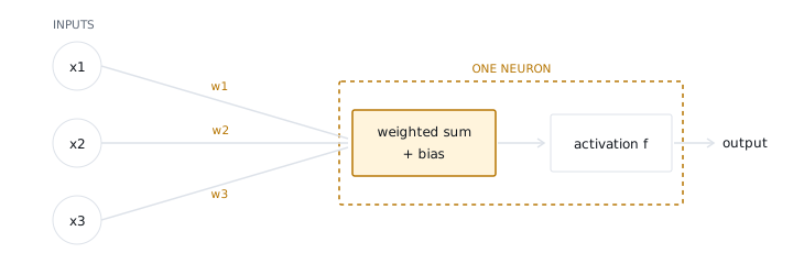
A neuron is a unit that multiplies each of its inputs by a weight, adds the products together with a bias, and passes the total through an activation function to produce one output.

Each part of that sentence names a quantity, and each one is defined below in the order it is used.

Inputs are the numbers a neuron receives. In this course inputs are always written as numbers, even when the underlying fact is a yes or a no. A yes-or-no input is coded as 1 for yes and 0 for no.

Consider a machine that decides whether an afternoon is suitable for going outside. It receives three inputs: the temperature, whether it is raining (1 for raining, 0 for not), and the wind speed.

A weight is a number attached to one input. It records two things at once: how much that input matters, and in which direction it pushes the answer.

A large positive weight on temperature means warmth pushes the answer toward yes. A large negative weight on rain means rain pushes the answer toward no. A weight near zero means that input is being ignored.

The bias is one extra number that belongs to no input. It is added to the weighted sum and sets how much total evidence is needed before the answer tips from one side to the other.

A large negative bias makes the neuron hard to convince. A positive bias makes it easy to convince.

The activation function is the rule that turns the single total into the output. The simplest activation function is the step: output 1 if the total is greater than zero, and 0 otherwise.

The full computation, written in words, is: multiply each input by its weight, add the products, add the bias, and apply the activation function to the result. Written as a formula with three inputs:

Worked example. Let the weights be 0.8 for temperature, −2.0 for rain and −0.3 for wind, with a bias of −0.1. Temperature and wind are given on a scale from 0 to 1. Take a warm day (0.9), no rain (0), light wind (0.2):

Now the same day, except that it is raining, so the rain input becomes 1:

Changing the rain input alone reversed the decision, because the weight on rain is large and negative compared with the other two weights. Every step of the calculation is multiplication, addition and a comparison with zero. The only open question is where the four numbers (three weights and a bias) came from, and that question occupies the rest of the course.

With two inputs the neuron can be drawn on paper. The neuron outputs 1 when the weighted sum plus bias is greater than zero and 0 when it is less. The border between the two answers is the set of points where the total is exactly zero.

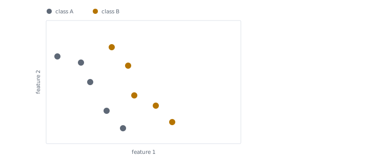
The decision boundary of a neuron is the set of input points where its total equals zero. With two inputs it is the set of points satisfying w1·x1 + w2·x2 + b = 0, which is the equation of a straight line.

A neuron with two inputs therefore divides the plane into two halves with a straight line and answers every question by reporting which side of the line the input falls on.

The weights and the bias do different jobs on that line.

1. The weights control the orientation of the line, which way it tilts. Change a weight and the line pivots.
2. The bias controls the position of the line. Change the bias and the line slides back and forth without rotating.

Training a single neuron is choosing where to put a line.

With three inputs the boundary is a flat plane cutting through three-dimensional space. With a thousand inputs it is a flat divide through thousand-dimensional space, which nobody can picture and which the algebra handles without difficulty.

A hyperplane is the general name for a flat boundary in any number of dimensions: a line in two dimensions, a plane in three, and the equivalent flat object beyond that. The one property to carry forward is that a hyperplane is always flat.

The total also carries information beyond its sign. Its size measures roughly how far the input point sits from the boundary. A point far inside the yes region produces a large positive total; a point barely on the yes side produces a total close to zero. The neuron is therefore reporting something like confidence, and the examples it is least sure about are the ones nearest the boundary.

The weights are not set by hand. In 1958 Frank Rosenblatt published a procedure that sets them from examples. The procedure shows the neuron one labeled example at a time. If the neuron gives the right answer, nothing changes. If it gives the wrong answer, the weights are nudged.

The perceptron update rule is the nudge. Write the true label as y and the neuron’s output as ŷ. For each weight, add a small step in the direction of the input, scaled by the error (y − ŷ). The bias receives the same step without the input factor.

The learning rate, written with the Greek letter η, is a small positive number that controls how big each nudge is. It appears in every lesson from here on.

The rule moves the boundary the right way for the following reason. Suppose the true answer was 1 and the neuron said 0. Then (y − ŷ) is +1, and a positive multiple of the input is added to the weights. That makes the weighted sum for this particular input larger next time, which pushes the total up toward positive, which is the answer that was wanted. When the error runs the other way, (y − ŷ) is −1 and everything happens in reverse. The rule contains no further cleverness: it leans in the direction of the answer it should have given.

Worked example. Start with both weights and the bias at zero, and set the learning rate to 0.5. The first example is x = (2, 1) with true label y = 1.

The full procedure repeats this over the whole set of examples, again and again, so that the line pivots and slides until no example is left on the wrong side.

1. Take the next labeled example.
2. Compute the neuron’s output.
3. If the output matches the label, change nothing.
4. If it does not, apply the update rule to every weight and to the bias.
5. Continue through the examples, and repeat the whole pass until a full pass makes no mistakes.

Linearly separable data is data whose two classes can be split by a single straight boundary. For linearly separable data the perceptron procedure is guaranteed to finish with every example on the correct side. This guarantee is one of the reasons the perceptron caused such excitement at the time.

The shape of the rule matters more than the formula. In Lesson 05 you will meet gradient descent, which does the same thing in a more general way: instead of reacting to a right-or-wrong verdict, it measures how wrong the answer was and steps downhill accordingly. That generalization is what makes training more than one layer possible.

Everything a single neuron can learn has the form “yes on one side of a straight divide, no on the other.” This limitation cannot be trained away, because it is built into the arithmetic of Section 02. It rules out a problem that is very small.

XOR (exclusive or) is the function of two inputs, each either 0 or 1, that outputs 1 when the two inputs differ and 0 when they match.

Plot the four points on paper and mark their outputs. The two zeros sit at opposite corners of the unit square, and so do the two ones. No single straight line can be drawn with both ones on one side and both zeros on the other. Try it for a minute; the attempt is the point. There is no such line, and therefore no choice of two weights and a bias produces one. XOR is not linearly separable.

XOR is small, but it is the smallest example of a very common situation: the categories of interest are not on opposite sides of any flat divide. Most problems worth solving look like this, which is why the limitation mattered so much. When Marvin Minsky and Seymour Papert laid it out in 1969, work on neural networks slowed for more than a decade. The field had the neuron and did not yet have a way to train more than one layer of them.

Be precise about what the limitation is, because this is the most common misunderstanding. It concerns the shape of the boundary, not the number of inputs. A neuron with a thousand inputs still draws one perfectly flat boundary through thousand-dimensional space. More inputs do not produce a bend.

The fix is therefore not a bigger neuron but more than one. In Lesson 02 you will see that two neurons, each drawing its own line, feeding a third that combines their two answers, separate XOR without difficulty.

A hidden layer is a set of neurons that sit between the inputs and the output, receiving the inputs and passing their own outputs onward. The two neurons in the middle of the XOR solution are a hidden layer, and once a network has one, the flatness limitation is gone.