Feature engineering is the work of deciding, by hand, which measurements of a raw input (such as a photograph) are turned into numbers and passed on to a classifier.

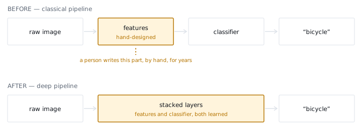
The classifiers studied in Grade 10 (support vector machines, logistic regression, decision trees) do not accept a photograph. Each accepts a vector of numbers. Before any learning can happen, somebody must decide which numbers. In 2008, a system that recognized whether a photograph contained a bicycle was built in two stages.

1. Feature extraction, designed by a person. The engineer reasons about what makes a bicycle look like a bicycle: two circular shapes of similar radius, a roughly horizontal bar between them, a certain density of thin straight edges where the spokes are. Code is then written to measure those properties: edge detectors, circle-finding transforms, histograms of the directions in which edges point. Real systems of the era used published feature extractors with names such as SIFT and HOG, each the product of years of research.
2. Classification, learned from data. The vector of measurements goes into the classifier, which learns a decision boundary between the classes.

The limit of this design is that the classifier can only be as good as the vector it is handed. If the features discard the information that distinguishes a bicycle from a motorcycle, no amount of training can recover it, because the distinction is no longer present in the numbers. The learning algorithm was not the bottleneck. The human choice of features was.

The human designer also had to anticipate every condition in advance: bicycles at night, bicycles at an angle, bicycles half-hidden behind a person, bicycles in the rain. Each failure meant returning to design another feature by hand. Each new problem domain (faces, handwriting, tumors, speech) meant starting over with a new team and a new set of extractors. The field was limited by a resource that does not scale: expert attention.

Representation learning is the alternative. The network learns the measurements itself, as part of training, instead of receiving them from a human. The feature-extraction stage becomes part of the model that trains.

The universal approximation theorem states that a network with a single hidden layer, if that layer is wide enough, can approximate any continuous function to any desired precision.

Taken alone, this theorem seems to make depth unnecessary. The theorem, however, guarantees only that a solution exists. It says nothing about how many units the hidden layer needs, and nothing about whether gradient descent can find the solution. For the kinds of structure that appear in real images, audio and language, the shallow solution can require an impractical number of units, while a deep network reaches the same function with far fewer. The reason is reuse: a feature computed in one layer is available to every unit in the layer above, so it is built once and used many times.

Inspection of a trained vision network shows a consistent pattern in what the layers respond to.

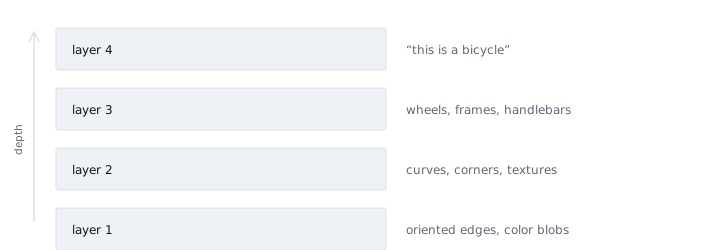
1. The first layer responds to oriented edges and color transitions.
2. The next layer combines those edges into corners, curves and repeating textures.
3. The next assembles those into recognizable parts: a wheel, an eye, a window frame.
4. Only near the top do units respond to whole objects.

Each layer writes its vocabulary in terms of the layer below it. A “wheel” detector is not built from raw pixels. It is built from curves, which were built from edges, which were built from pixels.

A feature hierarchy is this layered arrangement, in which each layer’s features are combinations of the features in the layer below.

Nobody designed the hierarchy. It is not in the architecture and not in the loss function. It is what minimizing error produces when the data itself is compositional.

Compositional data is data assembled from parts that are themselves assembled from smaller parts. Objects are made of parts and parts are made of edges; sentences are made of phrases and phrases are made of words.

The hierarchy emerges because the world is built that way. A deep network fits natural data well because its structure mirrors how natural data is assembled. Where compositional structure is absent, depth gives much less. This is why deep learning has transformed vision and language far more than it has transformed, for example, predicting next quarter’s sales from a spreadsheet of twelve columns.

Backpropagation was published in 1986. Convolutional networks that read handwritten digits were running in production on bank checks by the late 1990s. The core ideas of the Grade 11 course are therefore older than most teachers’ careers. Histories of the field nevertheless pivot on 2012.

Top-5 error is the fraction of test images for which the correct label is not among the model’s five most confident guesses. It is the standard score of the ImageNet competition.

In 2012 a network called AlexNet entered the ImageNet competition and cut the top-5 error rate from roughly 26% to roughly 15%. The improvement was so far outside the usual year-over-year change that it ended the argument about whether deep networks worked. AlexNet contained no new principle. It was the 1986 principle with three ingredients the earlier version never had.

Worked example. The size of the 2012 result, measured two ways:

1. Labeled data at scale. ImageNet supplied over a million labeled photographs across a thousand categories, assembled by crowdsourcing on a scale that was not possible before widespread internet participation. A deep network has a very large number of parameters, and parameters without enough examples simply memorize. The dataset was arguably the single most important contribution of the era, and it came from data collection, not from mathematics.
2. Compute of the right shape. Graphics processors were built to apply the same arithmetic to thousands of pixels at once. That is exactly the shape of a matrix multiplication, which is nearly all a neural network does. Hardware designed for video games was, in effect, hardware designed for deep learning, and a training run that would have taken months on a CPU came down to days.
3. Training techniques that keep gradients alive. In a deep stack, the gradients arriving from the loss shrink toward nothing before they reach the early layers, so those layers never learn. Three fixes addressed this: replacing saturating activations (such as the sigmoid, whose slope flattens to near zero for large inputs) with the ReLU, using dropout to resist overfitting, and initializing weights with care. They are unglamorous fixes, and they are the difference between a network that trains and one that does not.

Vanishing gradients are gradients that shrink toward zero as they are passed backward through many layers, leaving the early layers with almost no learning signal.

The ReLU (rectified linear unit) is an activation function that outputs its input when the input is positive and zero otherwise. Its slope does not flatten for large positive inputs, so, unlike a saturating activation, it does not shrink the gradient passing through it.

Dropout is a training technique that switches off a random subset of units on each training step, so that no unit can depend on any particular other unit being present. It resists overfitting.

Backpropagation itself was not among the missing ingredients; it had been available for twenty-six years. The decisive advance of the last two decades was not a cleverer equation. It was scale meeting an idea that had been waiting for it.

In deep learning, scale is a research result, not an engineering detail.

That pattern has repeated at least twice since 2012. It appears again in Lesson 6, with language models.

Each gain described above has a cost. A senior-level understanding includes being able to state the three costs without being prompted.

1. Depth is data-hungry. Removing the human from feature design means the network must discover the features itself, and discovery takes examples, often orders of magnitude more than a hand-engineered system would need. With two hundred labeled images, a classical pipeline with good features can still beat a deep network trained from scratch. Lesson 5 covers the standard escape from this problem.

2. Depth is expensive, in money and in energy. Training a large modern model consumes electricity on an industrial scale, and the cost falls on whoever can afford the hardware. That concentrates the ability to build frontier models in a small number of organizations, a technical fact with political consequences that Lesson 8 returns to.

3. Depth is opaque. In the classical pipeline the features could be read, and the reason for any decision could be stated exactly, because a person wrote the features. A learned representation carries no such guarantee. The network does have a reason, since it is a deterministic function, but that reason is distributed across millions of weights in no humanly readable form. When a deep model denies someone a loan or flags a medical scan as clear, “the network said so” is the accurate answer and an unacceptable one.

Interpretability is the degree to which a human can state why a model produced a particular output. Hand-written features are interpretable by construction; learned representations generally are not.

The rest of this course is a tour of what depth makes possible: convolution (Lesson 2), transfer (Lesson 5), attention (Lesson 6) and generation (Lesson 7). Each of those lessons also adds another item to this same bill.